Charge
Correction for iXPS (PDF version available here)
An iXPS data set
consists of a spectrum at
every pixel in an image. These spectroscopic image data sets may
exhibit
lateral differential charging as a consequence of:
- An
uneven X-ray flux
- Different intensity of
photoelectron
emission across the field of view
This is not
necessarily a problem for quantification where the limits of
integration
can be adjusted to accommodate
the charging. Neither is it a problem for peak fitting where peaks can
be fixed with respect to the primary peak which can be allowed to
move within limits.
However it is a problem for Principal Component Analysis (PCA) which is
used to improve the signal/noise in the iXPS data set. PCA recognises
different charge
shifts as a separate component increasing the number of components and
therefore the possibility that some will be lost in the noise of the
data. Correction of charging at every pixel is therefore necessary.
This page illustrates the steps required to do this.
The Sample
Islands
of silicon oxide, approximately 150 nm high, were created on
silicon by thermal oxidation followed by HF etching through a
lithographic mask.
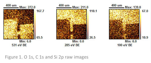
The Data
600
images of 256 x 256 pixels incremented in 1 eV steps from 600
eV to 0 ev were acquired over a 800 µm field of
view, at 160 eV pass energy with a dwell time of 100 seconds. The raw O
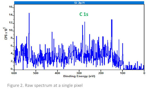
1s, C 1s and Si 2p images are shown in figure 1. The
images are converted to spectra, shown in figure 2, but the
signal/noise is not sufficient to allow accurate determination of the C
1s peak position.
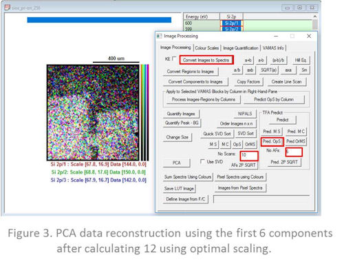
The
signal/noise must therefore be improved using PCA. The images are
overlaid and the first 10 components calculated, and the data then
reconstructed using only the significant components, in this case 6,
following optimum scaling. This is
accomplished by entering '10' in the 'No scans' field, '6' in the 'No
AFs' field followed by clicking the 'Pred OpS' button. When the PCA has
finished, the images are converted to spectra by clicking the 'Convert
Images to Spectra' button. The appropriate regions are highlighted in
red in figure 3.
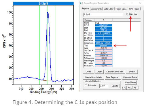
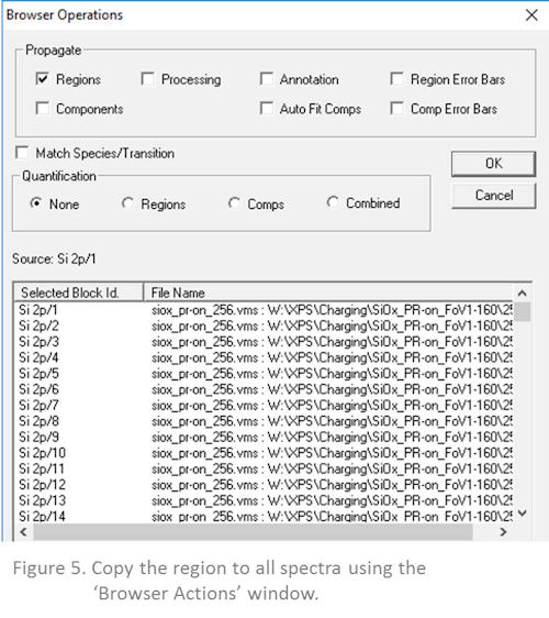
Tick
the 'Regions' checkbox, and press OK to
copy the region properties to all the spectra listed. Select all the
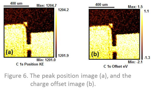
spectra and overlay them in the display pane. Clicking the 'Convert
Regions to Images' button, seen in the image processing tab of the
image processing window displayed in figure 3 computes an image
consisting of the C 1s peak position of each spectrum in kinetic
energy, shown in figure 6 (a). It is interesting to note that the thick
oxide has a higher kinetic energy that is lower binding energy, than
the native oxide, implying that the thick oxide is charging less. The
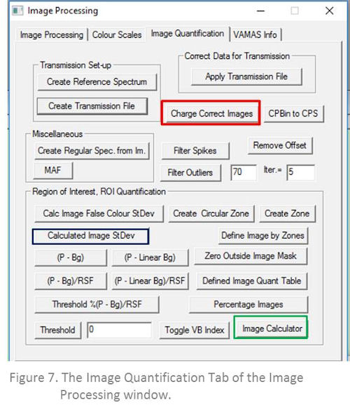
'Calculated Image StDev' highlighted
in blue is used to calculate the mean, standard deviation, maximum and
minimum values of the C 1s peak position. The charge offset image shown
in figure 6 (b) is calculated by subtracting the mean value from
figure 6 (a). This is accomplished by clicking the 'Image Calculator'
button, highlighted in green, and entering the following string 'vb0 -
[mean value]'. The reference is chosen as the mean value and not 285.0
eV, the value usually given to the C 1s hydrocarbon peak, because in a
three dimensional data set each spectrum must be shifted, since the
energy scale is common to all spectra and images will be lost as the
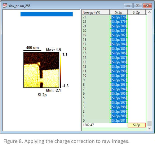
spectra are shifted. The charge offset image is then copied to the raw
data and displayed in the active window, as shown in figure 8. The
images to be corrected are highlighted and the 'Charge Correct Images'
button highlighted in red in figure 7 clicked. If more than one region
requires correction they must be corrected separately so that images
from one region are not transferred into a different region.
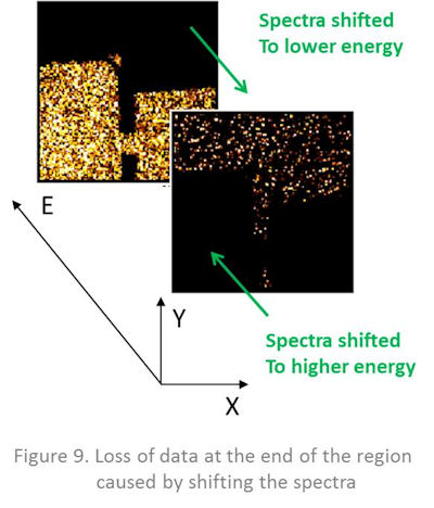
Figure
9 shows regions in the images containing zero counts as spectra have
been shifted. These images must be deleted from the data set, and the
maximum and minimum values of kinetic energy calculated with the image
standard deviation can help. The charge corrected data set should now
be saved. PCA should be carried out again to improve the signal/noise
in the charge corrected data set, following which further processing
such as quantification or peak fitting
may be undertaken.
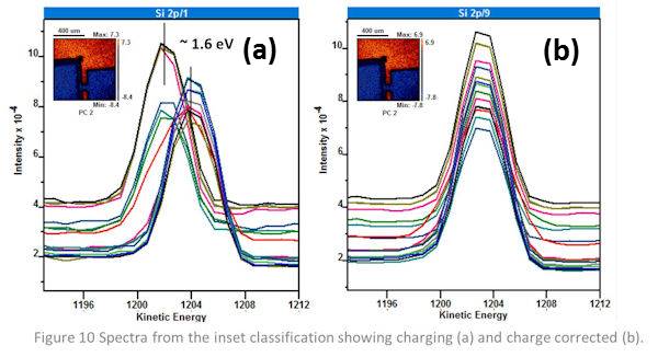
To illustrate the effectiveness of the charge correction procedure the
pixels in the second image principal component have been classified by
intensity into 16 segments, and the spectra in each classification
summed. Spectra from the raw data and charge corrected data are shown
figure 10 (a) and (b) respectively.
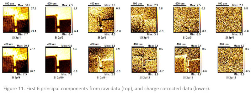
Figure
11 shows the first six image principal components from the raw data, top,
and from the charge corrected data, lower. There is
clearly more information present following charge correction. The loss
of information from the raw data is a consequence of charging resulting
in more components which are unable to be effectively separated from
the noise.
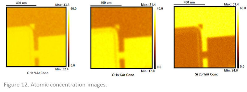
Figure
12 shows the carbon, oxygen and silicon atomic concentration images,
calculated from the photoelectron peak areas following correction for
the intensity/energy response of the instrument, and using Scofield
sensitivity factors. The images are plotted from zero intensity so as
not to show any misleading contrast. There is a higher carbon
concentration on the thermal oxide than the silicon/native oxide
surface, which most likely arises from remnants of the
photolithographic mask.
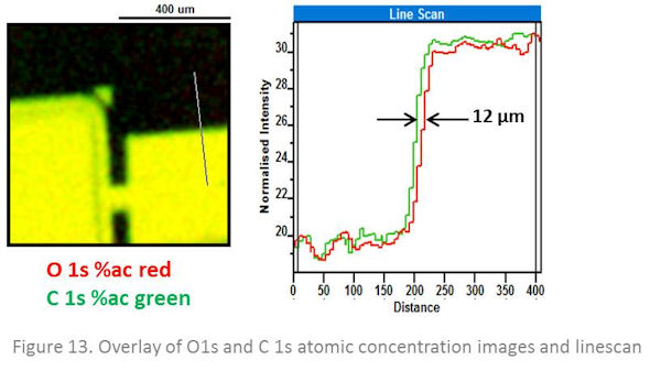
Figure
13 shows an overlay of the carbon and oxygen concentration images,
which reveals a line of carbon surrounding the thermal oxide,
consistent with the contrast seen in the higher order image principal
components. This arises from emission of C 1s photoelectrons from the
side wall of the thermal oxide. The line scan across the edge of the
thermal oxide shows the carbon extends 12 µm past the edge of the
oxide, which is consistent with the expected spatial resoluton of the
instrument at this field of view, and which couldn't be clearly
observed without charge correction of the spectroscopic image data set.